This will be my first technical article for my blog. The idea is to start a series of tutorials about optimization algorithms. In this post, I'll make a quick introduction to what is an optimization algorithm and then I'll talk about one specific that is, Particle Swarm Optimization (PSO).
What is an optimization algorithm ?
Optimization algorithms are here to solve optimization problems where we want to find the best solution within a large set of possible solutions.
Optimization problems are everywhere. For instance, when we enter a super market, the goal is to purchase all the things we need in a short time and with little expenses. Doing so we are optimizing our time and our budget.
We can define an optimization problem by three things:
- The measure of success (technically the cost function) which will be maximized or minimized.
- Instances of the problem which are the possible inputs to the problem, expressed in terms of design variables. These Instances can be subject to some constraints, thus setting bounds on the possible values to explore.
- The set of possible solutions which define the space to explore in order to find the best solution.
Generally, exploring the set of solutions is computationally heavy and very time consuming, that is why there are various algorithms to tackle these problems and find an appropriate and acceptable solution in a reasonable time.
These algorithms are iterative, and according to some criteria, one can decide whether the solution found is good enough to stop the optimization process. When that is possible, we speak about the algorithm convergence.
One of these algorithms is the Particle Swarm Optimization (PSO), which is the subject of this post. First, I'll try to explain how it works, then I'll walk you through a Python implementation, and test it on a real example.
What is Particle Swarm Optimization (PSO)?
PSO is an iterative optimization algorithm which tries to simulate social behaviour. It was developped by Dr. Eberhart and Dr. Kennedy, back in 1995.
It is best known that working together in order to achieve a goal is more efficient than no team work at all. PSO leverages this social behaviour by prevailing the information sharing between a set of possible candidate solutions, each called a particle.
A particle is defined by:
- A position. For example when the design variables are limited to two (i.e plane), a particle is defined by its coordinate (x,y).
- A velocity. This is a value used to move the particle position toward the best solution.
The information sharing is performed in two ways, giving two variants of PSO:
- Local PSO, in which the information sharing is between every particle and its direct neighbors. Here a particle's movement, at each iteration, is influenced by its local best known position. The particle and its neighbors form a ring data structure topology.
- Gloabl PSO, where the information sharing is between every particle and the best particle of all, defined by the best position. It is the best position which guides the movements of all the other particles, at each iteration. Here the particles are organized in a star data structure topology.
| Local PSO | Global PSO |
|---|---|
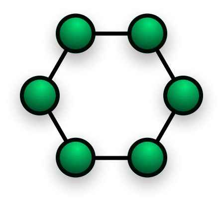 |
 |
Now that we understand how it works. Let's see the algorithm.
The Algorithm
We start by initializing randomly a population of particles in the search space. And through various iterations, each particle moves toward the best solution by following either the global best solution at each iteration or its locally best-known solution among its neighbors, depending on whether we consider local or global PSO.
Here is the pseudo-code for global PSO:
For each particle
    Randomly initialize its position and velocity
END
Do
  For each particle
      Calculate its fitness value (measure of success)
      If the fitness value is better than the best fitness value (pBest) in history
            Set current value as the new pBest
  END

  Choose the particle with the best fitness value of all the particles as the gBest
  For each particle
      Calculate particle velocity
      Update particle position using the computed velocity
  End
While maximum iterations or minimum error criteria is not attained
Python Implementation
The points to discuss here are the the initializations of the particle and their updates, both for the positions and the velocities.
- Particles are initialized randomly using a uniform distribution.
- The updates are performed using a slightly modified version of the initial paper, by the same authors (For further reading, go check this paper Inertia weight strategies in PSO).
Here is the python code which tries to implement a simple PSO:
import numpy as np

class PSO(object):
  """
    Class implementing PSO algorithm.
  """
  def __init__(self, func, init_pos, n_particles):
    """
      Initialize the key variables.

      Args:
        func (function): the fitness function to optimize.
        init_pos (array-like): the initial position to kick off the
                               optimization process.
        n_particles (int): the number of particles of the swarm.
    """
    self.func = func
    self.n_particles = n_particles
    self.init_pos = np.array(init_pos)
    self.particle_dim = len(init_pos)
    # Initialize particle positions using a uniform distribution
    self.particles_pos = np.random.uniform(size=(n_particles, self.particle_dim)) \
                        * self.init_pos
    # Initialize particle velocities using a uniform distribution
    self.velocities = np.random.uniform(size=(n_particles, self.particle_dim))

    # Initialize the best positions
    self.g_best = init_pos
    self.p_best = self.particles_pos

  def update_position(self, x, v):
    """
      Update particle position.

      Args:
        x (array-like): particle current position.
        v (array-like): particle current velocity.

      Returns:
        The updated position (array-like).
    """
    x = np.array(x)
    v = np.array(v)
    new_x = x + v
    return new_x

  def update_velocity(self, x, v, p_best, g_best, c0=0.5, c1=1.5, w=0.75):
    """
      Update particle velocity.

      Args:
        x (array-like): particle current position.
        v (array-like): particle current velocity.
        p_best (array-like): the best position found so far for a particle.
        g_best (array-like): the best position regarding
                             all the particles found so far.
        c0 (float): the cognitive scaling constant.
        c1 (float): the social scaling constant.
        w (float): the inertia weight

      Returns:
        The updated velocity (array-like).
    """
    x = np.array(x)
    v = np.array(v)
    assert x.shape == v.shape, 'Position and velocity must have same shape'
    # a random number between 0 and 1.
    r = np.random.uniform()
    p_best = np.array(p_best)
    g_best = np.array(g_best)

    new_v = w*v + c0 * r * (p_best - x) + c1 * r * (g_best - x)
    return new_v

  def optimize(self, maxiter=200):
    """
      Run the PSO optimization process untill the stoping criteria is met.
      Case for minimization. The aim is to minimize the cost function.

      Args:
          maxiter (int): the maximum number of iterations before stopping
                         the optimization.

      Returns:
          The best solution found (array-like).
    """
    for _ in range(maxiter):
      for i in range(self.n_particles):
        x = self.particles_pos[i]
        v = self.velocities[i]
        p_best = self.p_best[i]
        self.velocities[i] = self.update_velocity(x, v, p_best, self.g_best)
        self.particles_pos[i] = self.update_position(x, v)
        # Update the best position for particle i
        if self.func(self.particles_pos[i]) < self.func(p_best):
            self.p_best[i] = self.particles_pos[i]
        # Update the best position overall
        if self.func(self.particles_pos[i]) < self.func(self.g_best):
            self.g_best = self.particles_pos[i]
    return self.g_best, self.func(self.g_best)
We can test it on the sphere function, for example.
def sphere(x):
    """
      In 3D: f(x,y,z) = x² + y² + z²
    """
    return np.sum(np.square(x))

# If there is a main put this in the main
init_pos = [1,1,1]
PSO_s = PSO(func=sphere, init_pos=init_pos, n_particles=50)
res_s = PSO_s.optimize()
print("Sphere function")
print(f'x = {res_s[0]}') # x = [-0.00025538 -0.00137996  0.00248555]
print(f'f = {res_s[1]}') # f = 8.14748063004205e-06
Some points to discuss
- The initial point matters a lot in the performance of the optimization algorithm. As a rule of thumbs, as far as it is from the optmum, as long it takes the algorithm to converge (this is true for all optimization algorithms).
- PSO is a stochastic algorithm, the updates are performed using random processes. This can make it hard to track the solutions for multiple optimizatiion processes run. We can always use a seed for the random numbers though.
- It does not absolutely find the global optimal solution, but it does a good job finding one which is very close. For the sphere function, the global optimum is at (0, 0, 0), my implementation found another point which is not too bad.
- Depending on the number of particles, the convergence might take longer. Generally, it is better not to go beyong 50.
- For difficult functions, we might need more iterations before being able to find a good solution, between 500 and 1000 iterations.
This is the end of this long post. I hope it helps, I tried my best to keep it simple.
For a more advanced PSO, I highly recommend this open source python library Pyswarms. You can also find all the code on my github at My simple implementation.